Towards more energy efficient Machine Learning models

The third-generation neural networks

In recent years Machine Learning models evolved rapidly. Machine Learning is a popular field and data scientists and machine learning engineers have developed the most amazing models. From convolutional neural networks to deep Q-learning. All algorithms with applications in different kind of fields and which are used by most people around the anytime a day, while you are watching Netfix, using Google or check the wheather forecast.

Looking at the model architecture, these models might differ. Convolutional networks often have several pooling layers, simple ANN’s differ in number of hidden layers and are just straight forward and of course you can have RNN’s with LSTM units. Despite these differences they do have one thing in common. Before you can use them for predictions or recommendations they must be trained thoroughly. The training process is not a one time thing. Because models can change and new data is gathered through time this should be done periodically. This is often a long-lasting, very computational expensive process because training data might consist of hundreds of thousands elements. Nowadays this is not a real problem with all possibilities in hardware and cloud computing, using GPU’s etcetera. Although we have access to all these possibilities it still costs a lot of energy to train such a deep neural network. Energy that is scarce.

Isn’t there a way to train a model in more energy-efficient way?… There should be if we try to simulate the way our brain works since our brain uses much less energy than a standard laptop ¹.

Inspired by the human brain

And that’s exactly where Spiking Neural Networks got its inspiration from. I’m not a neurobiologist or neuroscientist but I will try to outline in a very simplified manner how networks in the brain basically work. Neurons communicate with each other via sequences of pulses. An action potential travels along the axon in a neuron and activate synapses. The synapses release neurotransmitters that arrive at the postsynaptic neuron. Here the action potential rises with each incoming pulse of neurotransmitters. If the the action potential reaches a certain threshold the postsynaptic neuron fires a spike itself ².

[https://medium.com/analytics-vidhya/an-introduction-to-spiking-neural-networks-part-1-the-neurons-5261dd9358cd] “Image of release of neurotransmitters to the postsynaptic neuron”

Spiking Neural Networks

How does it work and what are the challenges?

The question that immediately comes to mind is how to translate this principle into mathematical equations, an algorithm we can use to train neural networks. A second question is how to translate data, images or the handwritten digits from the MNIST dataset into spike trains.

Encoding

One way to translate images to spike trains is the use of a Poisson-encoding process ³,⁴, ⁵. Each image is encoded into a spike train and moves to the next layer in the network.

For example the BindsNET framework uses a Poisson enocoding method:

import os

from torchvision import transforms

from bindsnet.datasets import MNIST
from bindsnet.encoding import PoissonEncoder

# Load MNIST dataset with the Poisson encoding scheme
# time: Length of Poisson spike train per input variable.
# dt: Simulation time step.
dataset: MNIST(
    PoissonEncoder(time=250, dt=50),
    label_encoder=None,
    download=True,
    root=os.path.join("path_to_data", "MNIST"),
    transform=transforms.Compose(
      [transforms.ToTensor(), transforms.Lambda(lambda x: x * intensity)]
    ),
)

Decoding

The next step is to find out how to deal with these spike trains. Do we just count the spikes in a certain interval or do we wait until the first spike? These different decoding methods are all fine and different decoding methods work best for different tasks ²,⁶.

Modelling the neural dynamics

One aspect of the human brain described in the previous paragraph is that the action potential of a postsynaptic neuron rises with incoming spikes and the neuron releases a spike itself when the potential reaches a certain threshold. To incorporate these neural dynamics we need a mathematical model to describe this. An often used model is the Leaky-Integrate and Fire model that is a simplification of the Hodgkin & Huxley model which was designed originally for electrochemical engineering. It makes use of ordinary differential equations that are perfectly suited for the spike trains in the SNN’s ⁶, ⁷, ⁴.

Challenges

It is clear that the timing component of the spike trains is very important. This is also the biggest obstacle of the Spiking Neural Networks. The beauty of regular artificial neural networks is the contiuous process. The input is just a vector and this is multiplied for instance by a weight matrix, some bias is added and finally a sigmoid or relu function is applied. From input layer to output all continuous functions. This means we can apply gradient descent in the back propagation process. Here comes the spike train…a discontuous phenomenon. Very efficient since we only have to perform calculations when a spike train arrives, but gradient descent becomes a problem. This is the major reason why regulare ANN’s are still more popular. SNN’s are more complex and despite the energy efficiency, it all comes down to performance in terms of accuracy. That’s where ANN’s still win the game but SNN’s come closer and closer. It has been proven that SNN’s can be up to 1.900 times more efficient than classical RNN’s ⁶.

Frameworks

Although ANN’s are by far more popular scientists are doing more and more research on SNN’s and they are even developing complete frameworks for SNN’s. Two of those frameworks are both built on top of the famous ML library Pytorch: BindsNET and Spyketorch. Both have developed method to train SNN’s and are really easy in use ³, ⁸.

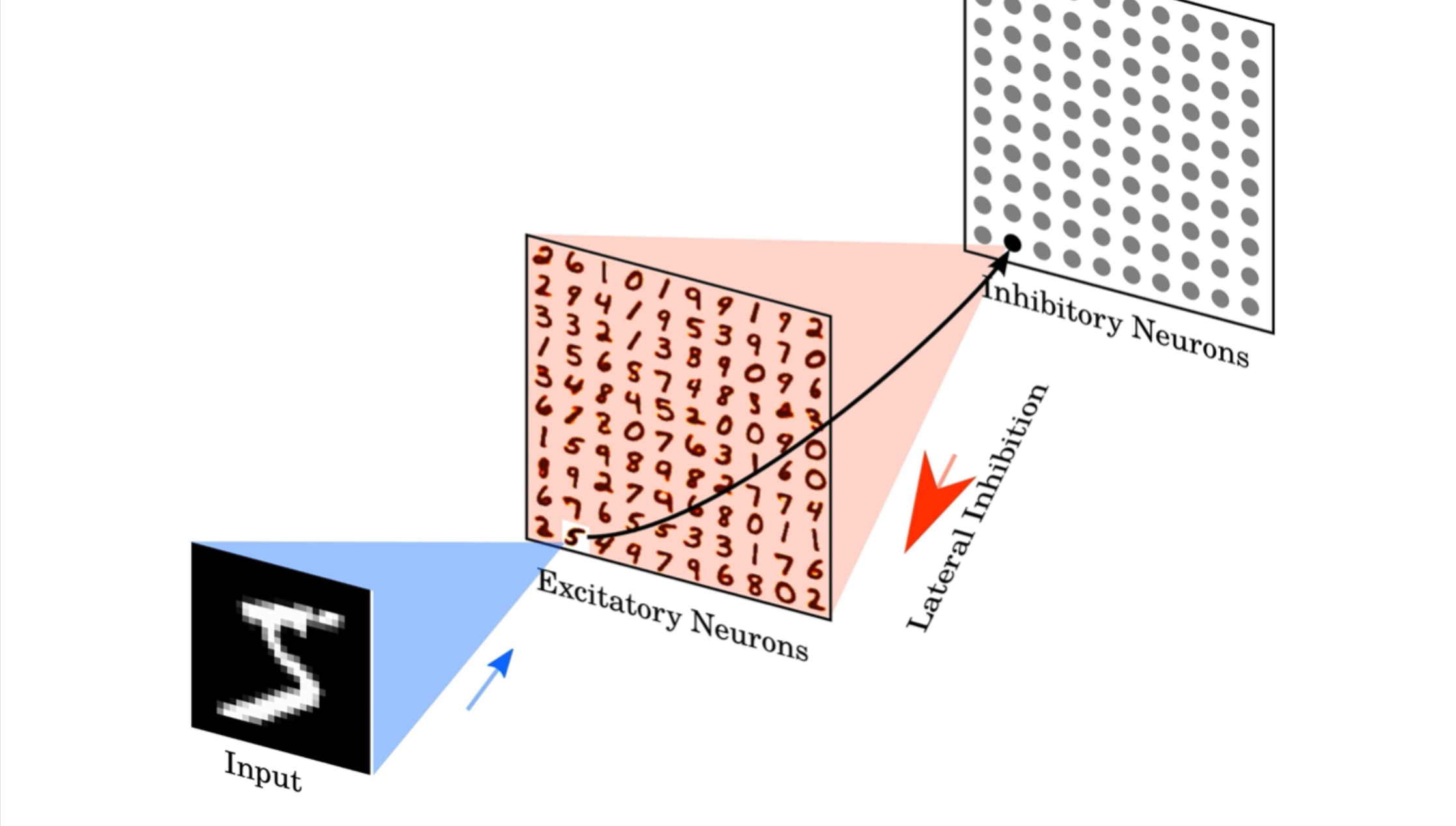
Let’s take again a quick look at the BindsNET framework. After setting the MNIST dataset BindsNET wants you to define a network object. We will follow the example as described on BindsNET github page and define a Diehl & Cook network.

from bindsnet.models import DiehlAndCook2015

# build Diehl & Cook network
network: DiehlAndCook2015(
  n_inpt=784,  # number of input neurons
  n_neurons=100,  # Number of excitatory, inhibitory neurons
  exc=22.5,  # Strength of synapse weights from excitatory to inhibitory layer
  inh=17.5,  # Strength of synapse weights from inhibitory to excitatory layer
  dt=1.0,  # Simulation time step
  nu=[1e-10, 1e-3],  # pair of learning rates for pre- and post-synaptic events, resp.
  norm=78.4,  # Input to excitatory layer connection weights normalization constant
  inpt_shape=(1, 28, 28))

The Diehl & Cook network consists in fact of two layers, the excitatory layer with excitatory neurons and the inhibitory layer with inibtory neurons. As you can see in the code snippet above the strength of these neurons is defined in the network setup ⁵.

The code above creates these layers with initial values for the connections between the layers. You can easily view the initial weights.

network.connections

results in:

{('X', 'Ae'): Connection(
  (source): Input()
  (target): DiehlAndCookNodes()
), ('Ae', 'Ai'): Connection(
  (source): DiehlAndCookNodes()
  (target): LIFNodes()
), ('Ai', 'Ae'): Connection(
  (source): LIFNodes()
  (target): DiehlAndCookNodes()
)}

which represent the connections between all three layers.

As you can see the inhibitory neurons are named LIFNodes() referring to the Leaky-Integrate and Fire model mentioned earlier.

You can also check the initial weights between the layers. Remember the strengths exc and inh we choose earlier in our network definition.

network.connections[("Ae", "Ai")].w

gives :

Parameter containing:
tensor([[22.5000,  0.0000,  0.0000,  ...,  0.0000,  0.0000,  0.0000],
        [ 0.0000, 22.5000,  0.0000,  ...,  0.0000,  0.0000,  0.0000],
        [ 0.0000,  0.0000, 22.5000,  ...,  0.0000,  0.0000,  0.0000],
        ...,
        [ 0.0000,  0.0000,  0.0000,  ..., 22.5000,  0.0000,  0.0000],
        [ 0.0000,  0.0000,  0.0000,  ...,  0.0000, 22.5000,  0.0000],
        [ 0.0000,  0.0000,  0.0000,  ...,  0.0000,  0.0000, 22.5000]])

where you can see again the usage of the PyTorch library in the data type tensor.

The observant reader will probably have noticed the connection from the inhibitory layer to the excitatory layer in the network.connections output above. Both layers influence each other in a slightly different way as can be read in ⁵.

Training

Training the models uses the PyTorch dataloader functionality to create a Python iterable over our dataset. So the next step would be to define this dataloader:

import torch

# Create a dataloader to iterate and batch data
dataloader: torch.utils.data.DataLoader(dataset, batch_size=1, shuffle=True)

Now the only that rest is train the network. Below you find the most basic code snippet to run the training process. Of course you can start with initial values for your neurons or add nice features to keep track of the progress.

for (i, d) in enumerate(dataloader):
    if i > n_train:
        break

    image: d["encoded_image"]
    label: d["label"]
    # Get next input sample.
    inputs: {"X": image.view(time, 1, 1, 28, 28)}
    # Run the network on the input.
    network.run(inputs=inputs, time=time, input_time_dim=1)

In the extensive documentation of the BindsNET repository and in their paper ³ you’ll find more great feautures.

At ODSC West 2021 I will talk in greater detail about these fascinating developments on SNN’s. More mathematical and technical details regarding the encoding and decoding methods will become clear. A solution for the gradient descent problem will be shown such as back propagation through time and surrogate gradients ⁶. Finally I’ll discusse the different approaches between the frameworks SpykeTorch and BindsNET.